Uncertainty is an inherent property of the subsurface world.
In reservoir modelling, every parameter carries a range of possible values. Nothing is fixed.
Experimental design is simply the systematic process of exploring that uncertainty by generating and running multiple scenarios, each based on different combinations of the uncertain parameters.
When specialized probabilistic or multi-realization software is available (such as MEPO or TNav's AHM license), this becomes straightforward.
But what if you don’t have access to software?
In this article, I walk you through a practical workflow to replicate a multi-realization study using only Excel and a lightweight supporting stack.
You will, of course, still need a reservoir simulator to actually run the cases.
At a high level, the process is straightforward:
The stack used here includes:
We need to run the cases with any simulator, but here we'll use the TNav simulation console to also demonstrate how to leverage its built-in Python scripting capability.
For this example, let's design a multi-realization study to understand the impact of uncertainty in relative permeability curves.
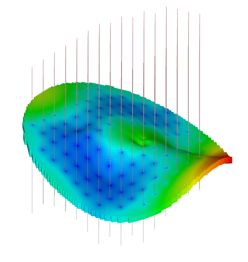
For the purposes of this study, the model itself is not critical. Here, I use a simple Coal Seam Gas (CSG/CBM) reservoir with 100 vertical wells.
We want to assess uncertainty in relative permeability, so the next step is to define the parameter ranges to explore.
For this example, we focus on relative permeability endpoints and Corey exponents for both gas and water phases. Rather than defining continuous distributions, we use discrete values for each parameter, which are then combined to generate individual realizations.
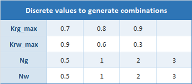
Combining all discrete parameter values using a full factorial design gives 3 × 3 × 4 × 4 = 144 unique cases.
At this stage, we are already envisioning the final visualization dashboard: an interactive production plot with buttons that let the user select specific values for each uncertain parameter and instantly update the displayed curves. This interactive dashboard is the end product we aim to produce with this workflow.
We create a 144-row table, each row a unique parameter combination. Easy to generate with the Claude add-in… takes seconds.
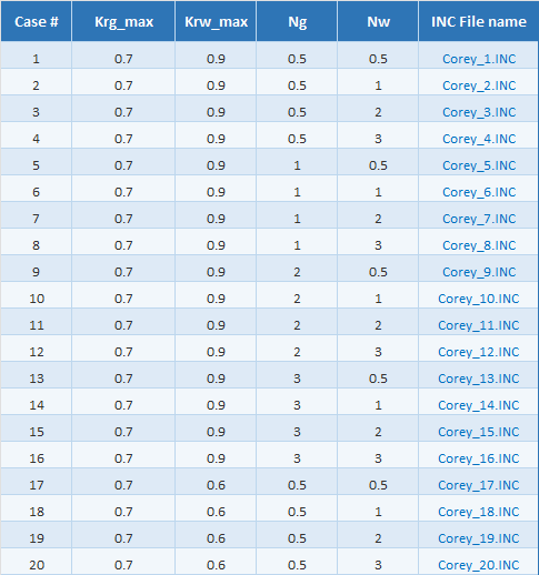
In this table, we add a final column containing the name of the INCLUDE file to be used in each simulation case. Each INC file defines the relative permeability curves for its corresponding parameter set.
For the content of the INC file, we could use tabulated data. However, since we are running with TNav, we instead use the Corey formulation via the COREYWG keyword, which provides a much simpler functional definition.
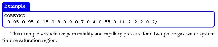
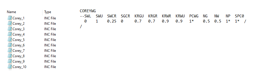
First, we create a template section in Excel containing all the required arguments for the COREYWG keyword:

A simple VBA macro then looped through all 144 cases. For each row, it pulls the corresponding parameter values, injects them into the template, and writes the resulting text block to an ASCII file, saved as “Corey_n.INC”.
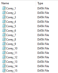
We end up with 144 INCLUDE files in our directory, each containing a clean block of text with the COREYWG keyword and its specific parameters.
The next step is to generate the simulation decks. As with the Corey INC files, we start by creating a table listing all cases along with their corresponding file names.
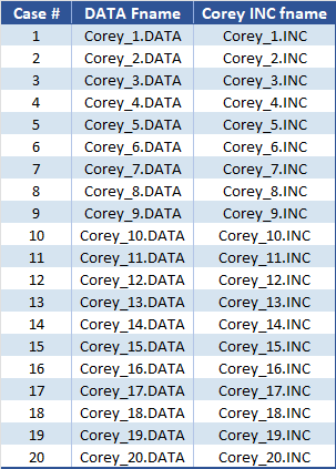
A second VBA macro then loops through each case. For every row, it retrieves the Corey INC file name and constructs an ASCII .DATA file by sandwiching it between two pre-prepared blocks:
[Block of text 1]
INCLUDE
'Corey_INC_Files/Corey_n.INC'
/
[Block of text 2]
Block 1 contains everything up to the INCLUDE statement; Block 2 contains everything after. The macro read each row, inserts the right reference, and saves the file under the case name.
Result: 144 ready-to-run .DATA decks.
If we were using Eclipse, we could generate a batch script to run each case via the command line, bypassing the launcher and any pre-processing application.
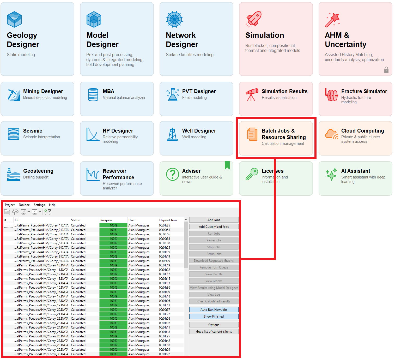
With TNav, we simply load all models into the batch queue and run them through its built-in batch functionality.
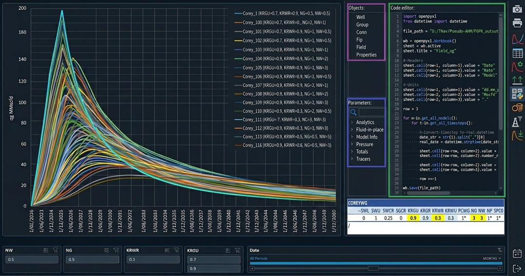
Once the simulations finish, we use TNav’s built-in Python code editor in the Graph Calculator to export all 144 production profiles into a single Excel file, with one click.
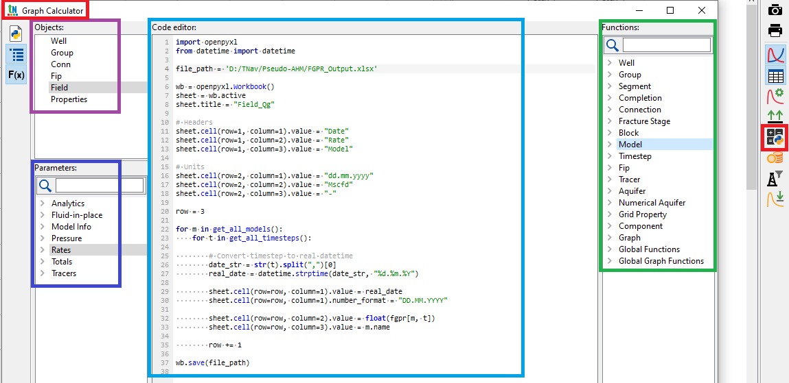
You don’t need to be a Python expert to create a script. Start from one of the scripts available in the TNav library, and ask Claude (or ChatGPT or any other LLM) to adapt it. TNav exposes objects, parameters, and functions that can be easily integrated into the code.
In this case, a quick look at the script shows that it writes to an external Excel file with three columns: date, rate, and model. The values are generated by looping through all models and all time steps.
The exported rate corresponds to the mnemonic FGPR, the field gas production rate vector.
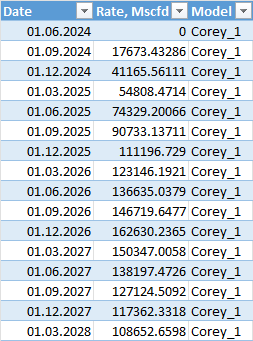
We run the script with a single click to generate the export file that looks like this:
Since we already had a master table with all the defining parameters for each case, we can now enrich the exported file by adding these parameters as additional columns, using lookups from the original table.
We also include a simple formula to generate a descriptive name for each case.
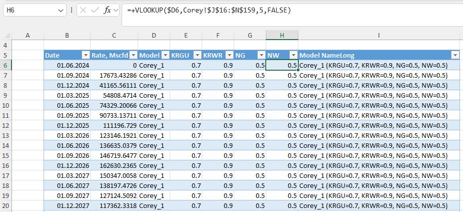
Why do this? Because in the next step, this table becomes the source for a pivot chart used to visualize and assess the impact of each parameter.
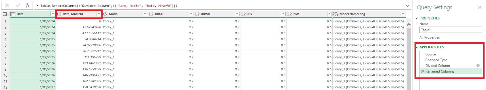
When this table is loaded into Power Query, the only transformation we apply is converting the rate from Mscfd to MMscfd and updating the header accordingly. That’s it.
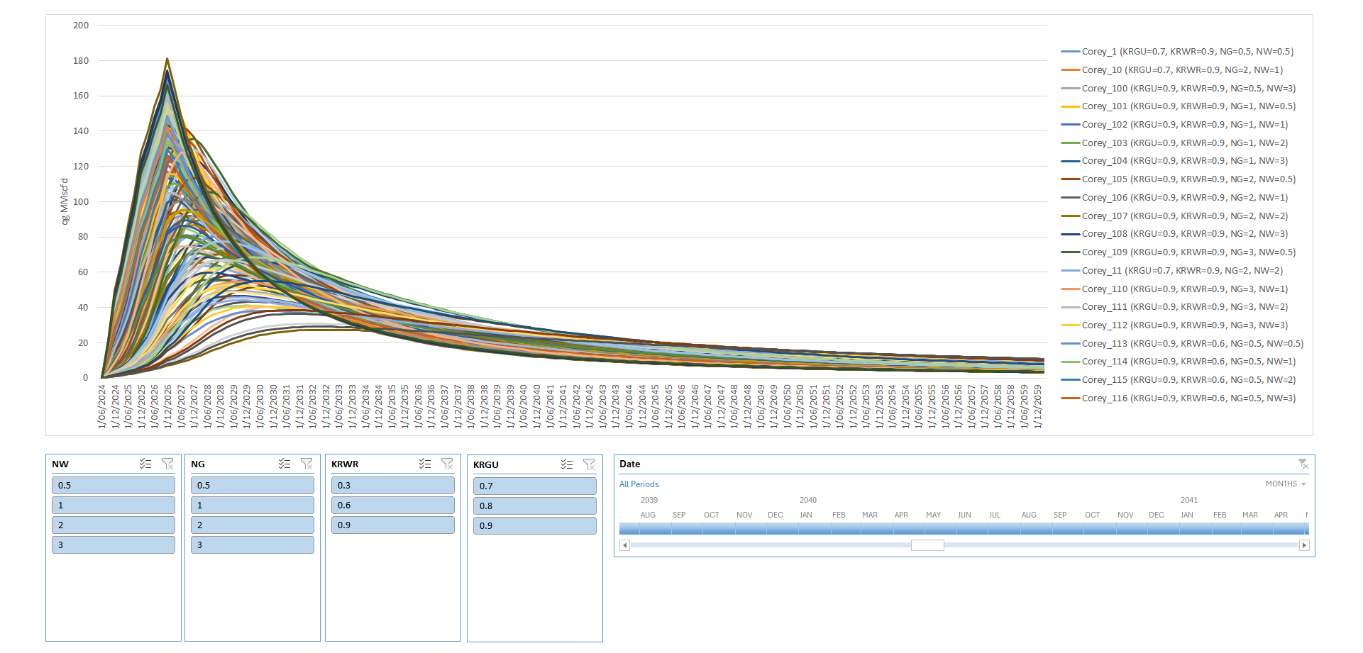
I then built a dashboard with a pivot chart and slicers for the four key parameters (rel perm endpoints and Corey exponents) plus a time slicer. This gave a clean, interactive way to explore sensitivities.
Here’s the full set of 144 cases:
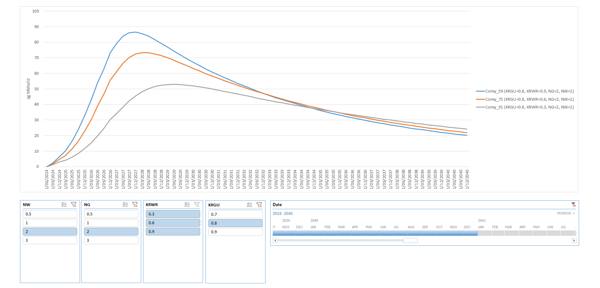
And here’s a sliced view showing gas production profiles up to 2040 (using the time slicer), isolating the impact of Krw_max (KRWR, all three buttons selected) while holding all other parameters at their base-case values (single buttons selected):
I’ve left the interpretation of these results and the discussion on relative permeability sensitivities for a follow-up article. The goal here was to show the mechanics of the workflow clearly and concisely.
Using only the TNav simulation console, we pre-processed multiple simulation decks with Excel and VBA, ran the full suite of cases, and leveraged TNav’s built-in Python scripting for a one-click export.
The results were then post-processed in Excel + Power Query into a user-friendly, interactive visualization dashboard.
In short: you can replicate a proper experimental design study with a simple, accessible stack: TNav (or any other simulator), Excel, VBA, Power Query, and Claude as your co-pilot for code and data tasks.
Explore a curated collection of valuable resources in our Store, both free and paid, all designed to help you upskill.
Alan Mourgues is a reservoir engineering consultant with 20+ years of international experience. He is the founder of CrowdField, a hub for subsurface professionals to explore practical tools, workflows, and new ways of working. Through CrowdField, he shares applied approaches, experiments with AI and automation, and surfaces real problems and solutions that translate into practical, usable outcomes.