You're staring at an infield development location. Your geological model says it's good. Mid-case economics look solid at $8MM NPV.
But… There's uncertainty, of course.
The low case is -$5MM. The high case, $25MM.
The debate: should we spend $1.5MM on 3D seismic first?
This is a classic Value of Information (VOI) problem. It's not about whether this data is "nice to have"… it always is. It's about whether the information it provides is worth more than it costs. And the tool to answer that question rigorously is Bayes' theorem.
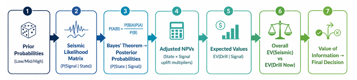
Let’s walk through a complete Bayesian VOI analysis, and see exactly how to quantify whether that seismic survey pays for itself. No gut feel. Just structured decision analysis.
Before we run any Bayesian math, let's define the problem structure.
Every VOI analysis starts with two things:
In our case, the states of nature are three possible well outcomes, each with an associated NPV from an external economic model:
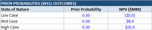
These prior probabilities reflect our current belief about the subsurface. They come from a joint geoscience/engineering assessment of the subsurface-turned-to-revenue system.
Our two decision alternatives are straightforward:
The expected value of drilling now is simple arithmetic:
EV(Drill Now) = (0.30 × -$5) + (0.50 × $8) + (0.20 × $25) = $7.50 MM
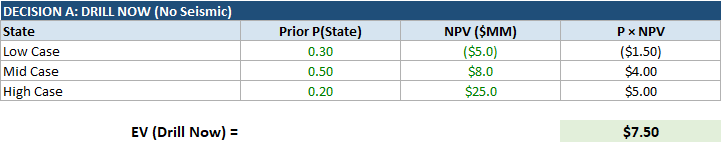
This is our baseline. The expected value of the project using today's information alone. Every VOI calculation is measured against this.
Now, why does shooting seismic change your expected value?
The low-, mid-, and high-case outcomes don't change. What changes is our understanding of which outcome is more likely.
Strictly speaking, new information can also affect the outcomes themselves. Better structural imaging and reservoir characterization may lead to improved well placement and therefore different NPVs. For now, however, we will focus only on the probability update and revisit the impact on NPV later in the analysis.
Because the seismic survey provides new information, what we need to work out is this:
What is the probability of the high, mid, and low cases after we shoot seismic?
In other words, how do we estimate the posterior probabilities?
Enter Bayes.
Let’s work backwards from the destination we want to reach, which is:
... AFTER we shoot seismic.
Here's the crux of the problem: seismic doesn't tell us the answer. It gives us a signal, and that signal is imperfect.
A "strong" signal does not guarantee a High Case outcome.
A "poor" signal does not mean the prospect is worthless.
The seismic response itself is subject to what is called a reliability or likelihood matrix, which shows how the observed signal depends on the underlying state of nature.
In practical terms, it answers the following question:
If the true state of the project is Low, Mid, or High, what is the probability that seismic would indicate a Weak, Neutral, or Strong signal?
P(Signal | State):
This likelihood matrix is a key input to the Bayesian analysis, and is typically calibrated from offset well results, seismic modelling, analogues, or expert judgement.
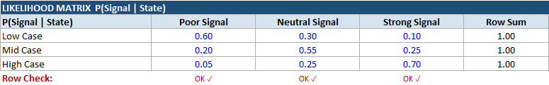
Read the matrix row by row. For example, if the true state is the Low Case, there is a 60% probability that seismic indicates a Weak signal, a 30% probability it indicates a Neutral signal, and only a 10% probability it indicates a Strong signal.
This asymmetry is what gives seismic its diagnostic value. If every row looked similar, the seismic response would contain very little information and would behave almost like random noise.
Note: the terms poor / neutral / strong signal are intentionally mapped to the seismic ability to correctly diagnose the low / mid / high cases respectively. In other words, a “poor signal” should be interpreted as “seismic indicating the low-case state,” while a “strong signal” means “seismic indicating the high-case state.” The terminology is relative to the underlying state of nature being diagnosed, not to seismic quality itself.
The likelihood matrix should therefore be read as: “if the true underlying state is the low-case outcome, what is the probability that seismic correctly indicates that low-case state?” The same logic applies to the mid and high cases.
The challenge now is that these are not the probabilities we are looking for.
The likelihood matrix tells us the probability of observing a seismic response given the true state:
P(Signal | State)
What we actually want are the posterior probabilities:
P(State | Signal)
In other words:
Given the seismic response we observe, what is the updated probability that the prospect is actually Low, Mid, or High?
This is where Bayes’ theorem comes in. It “inverts” the likelihoods using the formula:

You can think of Bayes as a probability translation machine.
It converts:
into:
That is the whole point.
Let's understand all terms in Bayes' equation, one by one:
P(State) is the prior probability.
It means: What did we believe about the state before seeing the seismic result?
P(Signal | State) is the conditional probability, also known as the likelihood.
It means: If the true state is known, how likely are we to observe a particular seismic signal?
P(State | Signal) is the posterior probability.
It means: After observing the seismic signal, what is the updated probability of each state?
This is what we ultimately want to solve for. It appears on the left-hand side of Bayes' equation.
P(Signal) is the marginal probability of the signal.
It means: What is the overall probability of observing this seismic signal, across all possible states?
For example: "What is the probability that seismic indicates a Strong signal, before knowing the true state of the reservoir?"
We calculate it by considering every possible way a Strong signal can occur:
P(Strong)
=
P(Strong | Low) × P(Low)+P(Strong | Mid) × P(Mid)+P(Strong | High) × P(High)
Looking at the reliability matrix (left terms) and the prior probabilities (right terms), we obtain:
P(Strong)
=
(0.10 x 0.3)
(0.25 x 0.5)
(0.70 x 0.2)
=
0.295
This is an unconditional (or absolute) probability, but in Bayesian statistics, it is commonly referred to as the marginal probability or evidence term.
We can compute the marginal probabilities for all seismic responses using the following matrix:
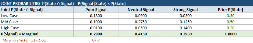
Notice that a marginal probability is simply the sum of the relevant joint probabilities. For example:
P(Strong)
=
P(Low∩Strong)
P(Mid∩Strong)
P(High∩Strong)
where, by definition, the joint probability is: :
P(State∩Signal) = P(Signal∣State) × P(State)
This represents the probability that the reservoir is in a particular state (Low, Mid, or High) and that seismic indicates a particular signal (Weak, Neutral, or Strong).
Importantly, this joint probability is exactly the numerator of Bayes' theorem:
P(Signal | State) × P(State) = P(State ∩ Signal)
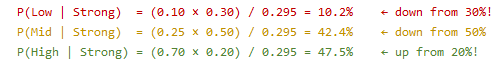
Now, putting together all the terms in Bayes' equation for a Strong seismic signal:
That's the magic.
A Strong seismic signal more than doubles the probability of the High Case (20% → 47.5%) and reduces the probability of the Low Case from 30% to 10.2%.
The signal does not eliminate uncertainty. It concentrates it.
And concentrated beliefs lead to better decisions.
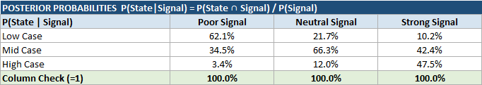
Applying Bayes' theorem to all possible seismic outcomes gives us the full set of posterior probabilities:
To focus on the Bayesian probability update, we have assumed so far that the NPVs themselves remain unchanged and that only the probabilities are updated after shooting seismic.
In reality, however, new information can affect more than just our beliefs.
Better structural imaging, improved confidence in reservoir quality mapping, and a clearer understanding of fluid distribution may allow us to optimize well placement and target the sweet spot more effectively.
This can translate into improved recovery, higher production rates, and ultimately a different NPV.
In other words, seismic can change not only the probability of success, but also the value of success.
We capture this effect through NPV uplift multipliers: a (State × Signal) matrix that adjusts the base NPV for each combination of reservoir state and seismic response.
In practice, these uplift (or downside) factors would typically be derived from well placement optimization studies, multiple development scenarios, reservoir simulation forecasts, analogue field performance, or history-matched models that quantify the impact of improved (or degraded) structural definition and reservoir characterization.
Here is the matrix used in this example:
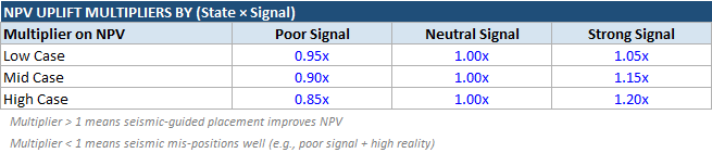
A multiplier > 1 means seismic-guided well placement adds value. A multiplier < 1 means the signal misleads (e.g., a poor signal in what is actually a high-case reality could lead to a suboptimal well path).
This matrix encodes both the upside of good information and the downside risk of misleading information.
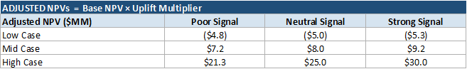
From our original NPV estimates for each state, we apply the NPV uplift multipliers shown above:
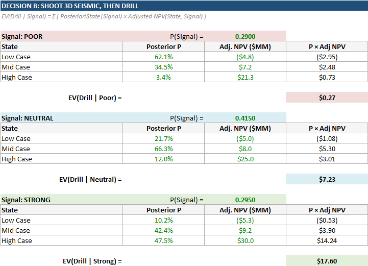
We can now compute the expected value of drilling for each possible seismic outcome:
EV(Drill | Signal) = Σ [ P(State|Signal) × Adjusted NPV(State, Signal) ]
In words:
The expected value of drilling after observing a particular seismic signal is the sum of the adjusted NPVs, weighted by their corresponding posterior probabilities.
Here is the expected value of drilling for each possible seismic outcome:
Summarizing the above:

The overall expected value of the seismic strategy is obtained by weighting each conditional expected value by the marginal probability of observing the corresponding seismic signal:
EV(Seismic)=Σ [P(Signal)×EV(Drill∣Signal)]
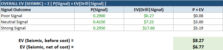
Note: In the example above, seismic acquisition cost is treated separately from the project NPVs and is deducted after computing the expected value of the seismic strategy.
If the input NPVs already include seismic acquisition cost, this final deduction should not be applied to avoid double counting.
At this point, we have everything we need to evaluate whether shooting seismic creates value.
Without seismic, our best estimate of project value is simply the expected value of drilling today, based on our prior probabilities.
With seismic, we gain information before committing to a drilling decision. That information allows us to update our beliefs, reassess the expected value of the opportunity under each possible seismic outcome, and then weight those outcomes by their probability of occurrence.
The difference between these two strategies is the Value of Information (VOI).
The table below compares the expected value of drilling immediately against the expected value of the seismic-informed strategy and calculates the resulting value of information.
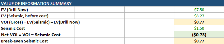
In other words, the ability to update our beliefs and make better decisions based on the seismic results adds $0.77 MM of expected value to the project, before paying for the survey itself.
That is the essence of VOI: The information is worth $0.77 MM. If a vendor could provide identical information for $0.50MM, you should buy it. If the same information costs $1.50 MM, you should not.
In this example, the answer is No.
The seismic survey creates value by improving our understanding of the subsurface and enabling better-informed decisions. The analysis shows that the information provided by the survey is worth $0.77 MM in expected value.
However, the survey itself costs $1.50 MM (acquisition, processing, and interpretation), resulting in a net Value of Information (VOI) of -$0.73 MM.
From a purely economic perspective, the rational decision is therefore to drill immediately rather than acquire seismic first.
Importantly, this does not mean the seismic survey has no value. Quite the opposite. The information is worth $0.77 MM. The issue is simply that the cost of acquiring that information exceeds the value it creates.
The break-even seismic cost, that is, the maximum amount we would rationally be willing to pay for the information, is therefore $0.77 MM. At any cost below that threshold, the seismic survey would generate positive net value.
Of course, this conclusion is highly sensitive to the underlying assumptions. Change the prior probabilities, the seismic reliability matrix, the NPV estimates, the uplift factors, or the seismic cost, and the recommendation may change completely.
This is one of the key limitations of any Value of Information analysis. The mathematics is relatively straightforward; the real challenge lies in estimating the inputs with sufficient confidence.
For that reason, the greatest value of the exercise is not the specific recommendation itself. Rather, it is the framework it provides for thinking rigorously about uncertainty, information, and decision-making under uncertainty.
The Bayesian VOI approach does not replace geological or engineering judgement. It complements it. It forces teams to make assumptions explicit, test them systematically, and understand exactly which uncertainties matter most and where additional information is likely to create value.
---
A couple of important caveats are worth noting.
First, this analysis assumes that drilling proceeds regardless of the seismic outcome. In practice, a seismic survey creates not only information, but also optionality.
After observing the seismic response, a decision maker may choose to drill, defer, farm out, acquire additional data, or walk away altogether.
That flexibility can materially increase the Value of Information by avoiding poor outcomes and preserving capital for better opportunities., and is not captured in the simplified example presented here.
Second, the results are highly sensitive to the underlying assumptions.
Prior probabilities, seismic reliability estimates, NPV forecasts, uplift factors, and seismic acquisition costs all influence the outcome. Change the inputs, and the answer can change.
In Part 2, I will extend the framework to include a full post-seismic decision tree with a walk-away option, as well as a sensitivity analysis on the key assumptions.
The objective will be to explore not only the expected value of information, but also the robustness of the recommendation and identify which uncertainties matter most to the decision.
Explore a curated collection of valuable resources in our Store, both free and paid, all designed to help you upskill.
Alan Mourgues is a reservoir engineering consultant with 20+ years of international experience. He is the founder of CrowdField, a hub for subsurface professionals to explore practical tools, workflows, and new ways of working. Through CrowdField, he shares applied approaches, experiments with AI and automation, and surfaces real problems and solutions that translate into practical, usable outcomes.